In which your hopeful protagonist describes Million Point Sculptures, and a highly interactive exploration tool written in Metal.

In the 1980s there was a wave of fascination with fractals and chaos in popular culture, and several books really caught the imagination of young me.

One was Chaos by James Gleick (un classique)¹. Also there were some lovely books by Clifford Pickover, like Computers and the Imagination, containing curious things like Million Point Sculptures: intriguing generated art showing wispy smoke-clouds. They’re generated by some quite simple equations.

Clifford’s most well-known MPS equation is this classic 2D one:

$$ \begin{aligned} x_{n+1} &= \sin(a\,y_n) + c \cos(a\,x_n) \\ y_{n+1} &= \sin(b\,x_n) + d \cos(b\,y_n) \end{aligned} \label{eq:clifford_classic} $$

To plot this MPS: choose some parameters \( a \) and \( b \) (which dictates the shape), and a starting point for \( (x_0, y_0) \),² and iterate the equation many times. We leave a faint mark on the pixels we visit as we go, building up the shape.

Another Clifford equation is a 3D variation:

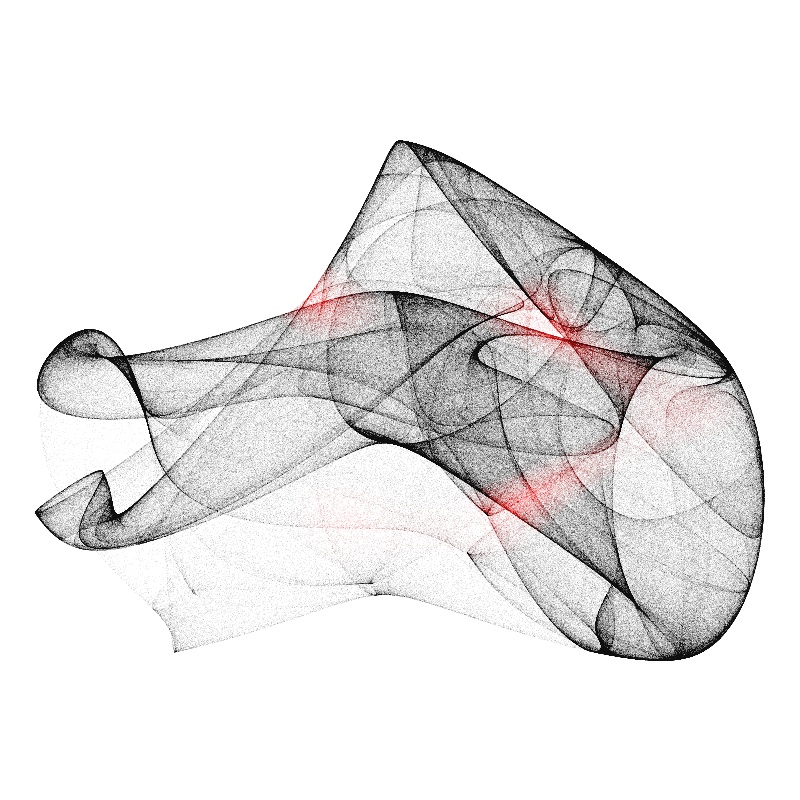
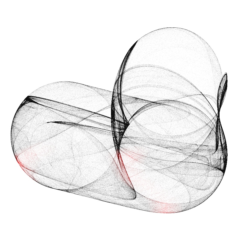
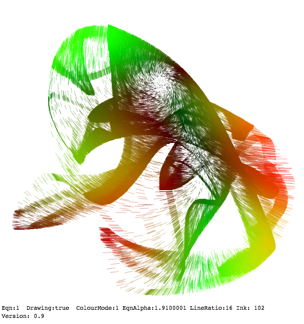
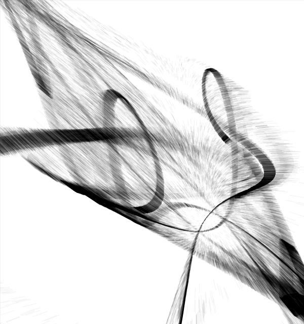
$$ \begin{aligned} x_{n+1} = \sin(a\,y_n) - z_n \cos(b\,x_n) \\ y_{n+1} = \sin(b\,z_n) - x_n \cos(c\,y_n) \\ z_{n+1} = \sin(c\,x_n) - y_n \cos(a\,z_n) \end{aligned} \label{eq:clifford_3d} $$

This is the system I played with the most. Here’s some of my original image generations from around 20 years ago:

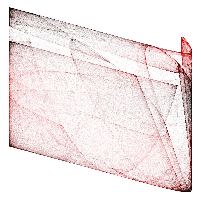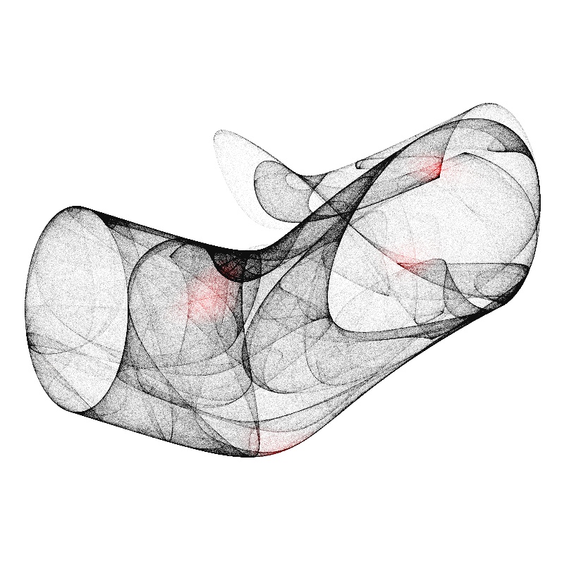The above were implemented in straightforward Python (slow). The touches of colour are my own embellishment (I can’t remember the rule).

They’re not large resolution renders but I really like the grittyness of the pointillism look.

I also wrote a Processing sketch back then to allow some jamming on rendering ideas; a few results below.

Writing a modern MPS explorer: Ynfold

I recently went back to look at Million Point Sculptures again. I’ve retired the Python script and I’m writing an interactive app called Ynfold (‘in-fold’) using Apple’s Metal (and SwiftUI). It allows real-time exploration and can animate MPS in real-time.

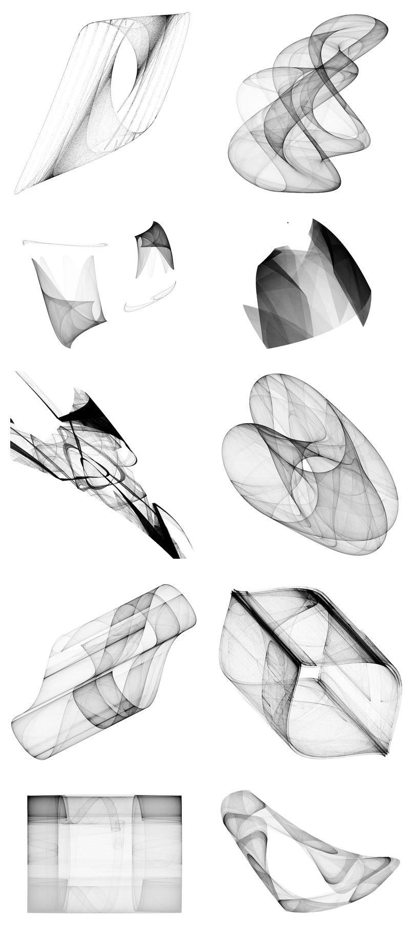
Some of the shapes I’ve spied so far:

Benefits of an interactive MPS tool:

Real-time MPS animation

It’s lovely and swirly and 60 fps.

Rapidly find (and hone) transient beauty

People tend to focus on the obvious cloud shapes, but there are some very interesting other things going on in MPS. They can pass by in the blink of an eye however:³

• line-art
• exploding ribbons
• exploding tiny clouds/copies
• rare “smooth shading” effects (overlapping, gentle shading)
• galaxy/nautilus images during the ‘settling’ part of the iterations (if you have settle iterations > 0, you might entirely miss these)

A blunt tool like a python script makes these things much harder to find and play with – or you might not realise that they’re even there.

Generate print-ready images with correct exposure

A bog-standard MPS script can easily generate on-screen or on-disk images. But if you want a high DPI image for printing, there are annoyances:

• correctly ‘exposing’ your MPS at print resolutions: if you want to render your MPS image scaled by factor \( S \), you need to adjust exposure by a factor of \( S^2 \), the same principle as in photography⁴
• faffing with getting correct aspect ratio for the design you want to print: an interactive tool can deal with this really nicely by making the interactive viewport be the correct aspect ratio for the print.

Why implement in Apple Metal?

I’ve done quite a bit of GL/GLSL in the past, but it’s just not the tool for this; GLSL is well suited to single pixel pipeline problems that don’t need to share state with other parallel computation. But the MPS algorithm involves a notional pixel hopping all over the display, leaving traces as it goes. Not a good fit!⁵

Compute platforms like Metal (and Vulkan etc.) are much better suited to this: the foundation is more based on general work in threads (and thread groups), with access to shared memory (with synchronization primitives).

This more general mode of GPU computation also means it is much easier to shoot yourself in the foot!

(I want to try out Vulkan some time. For this project, right now, Metal is the correct choice: it’s more opinionated and there’s a shorter path to what I want to achieve.)

How Ynfold works

It’s a dual MacOS and iPadOS using the Metal API. It’s fairly straightforward but there are some interesting little details.

Every pixel on the display gets its own worker thread (using threadgroup dispatch), and has access to atomic-access shared memory for the final image (histogram). A thread executes \( n \) iterations of the equation system, incrementing the shared histogram count for each pixel it visits.

The Metal kernel is split into obvious functions: one is a walker that loops through all iteratations for a coordinate. Another function does tone mapping of the result with a bog standard \( 1 - exp(-m * \mathrm{count_max}) \) function.⁶

Subtleties of Metal implementation

Avoiding contention: if all the worker threads starting iterating at the same coordinate then the contention on the shared histogram is going to be hideous. So we randomise the starting coordinate with a hash on the thread ID and a seed (that is incremented every frame).⁷

Dealing with slowdown due to contention: if you find something of interest and it has an attractor with points closely packed around it, the contention on the histogram ramps up. You get sluggish UI or, worst case, my mac actually freezes. This can be dealt with by more sensibly scheduling work (think of it as adding yields), and maybe by exiting a worker early if we think wise.

Choice of RNG: I’ve added a choice of hashing algorithms to the app (for generating the pseudo-random numbers) and it usually doesn’t make much difference that I can see. There have been some marginal cases where changing the RNG has increased the exposure a bit on a challenging render. But normally the computationally cheapest works fine (LCG or XORshift).

Ynfold

The app is working pretty well but not released at this time (polish needed). Watch this space!

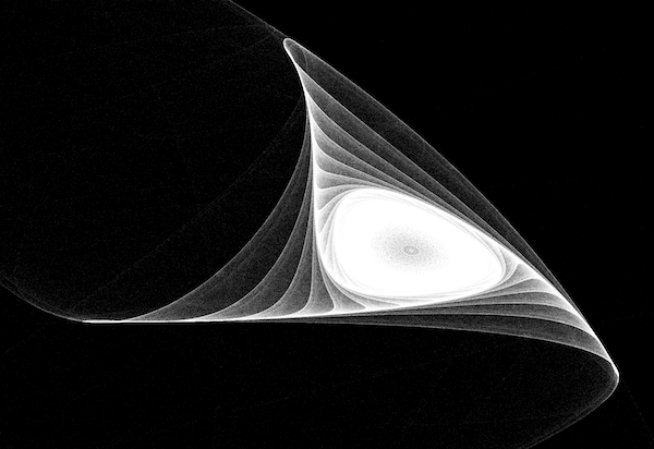
There’s another post coming soon that will cover some results of using the app, including the ‘focus’ concept in MPS systems, where some parameter constraints give you consistent shape outlines (geometric invariants).

Until then, here’s an example focus image.

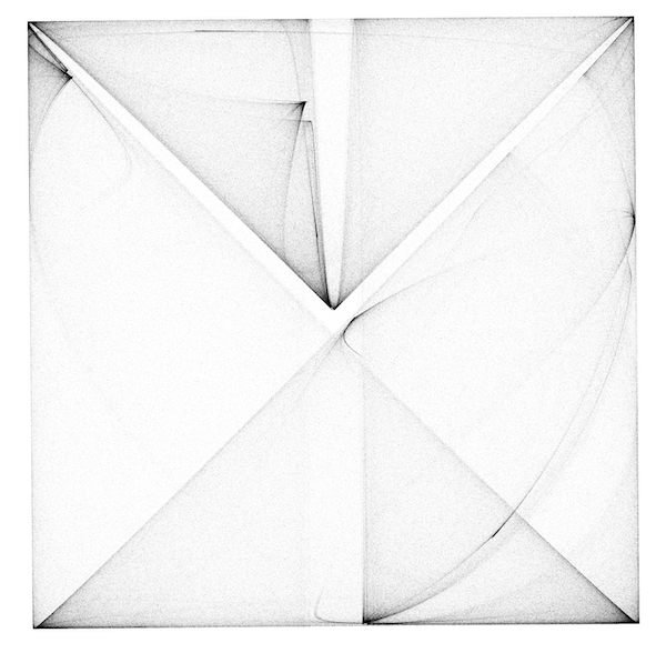
I think it must be an x-ray of an envelope.

Details for budding point-o-nauts

Experimentation guide: distilling the equations

Typically you see MPS equations using both sin and cos functions. If you’re experimenting with trying different equations you might try changing the trig functions, raising them to powers, and also change the signs (-/+) inside and outside the functions. Unfortunately, this is a fine way to end up wasting time by unknowingly trying the same thing multiple times because sin and cos are so closely related:

$$ \begin{aligned} \operatorname{sin}(x) &= -\operatorname{sin}(-x) \\ \operatorname{sin}(x + \pi) &= \operatorname{sin}(-x), -\operatorname{sin}(x) \\ \operatorname{sin}(x + \pi / 2) &= \operatorname{cos}(x), \operatorname{cos}(-x) \\ \operatorname{sin}(x - \pi / 2) &= -\operatorname{cos}(x), -\operatorname{cos}(-x) \\ \end{aligned} $$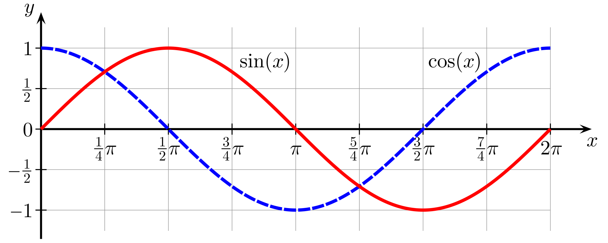

The way to avoid wasted effort and maintain sanity is to only use sin (never cos), and only do addition of your main terms (never subtraction), and use angle offsets to represent the function and +/-.⁸

Example: here’s the classic Clifford 2D MPS \eqref{eq:clifford_classic} written using angle offsets and only sin:

$$ \begin{aligned} x_{n+1} &= \sin(a\,y_n) + c \sin(a\,x_n + \pi / 2) \\ y_{n+1} &= \sin(b\,x_n) + d \sin(b\,y_n + \pi / 2) \end{aligned} $$

This form obviously also allows you to use arbitrary angle offsets like \( \pi / 4 \).

Recipe for generalised MPS exploration

For this you need a formalised idea of an MPS equation system (in order to enumerate over different systems).

Suppose you have an MPS equation system with \( d \) axes (dimensions) and \( n \) terms in each equation.

Then your equation system has a grid of \( dn \) terms, with each term being something like this:

$$ \begin{aligned} (-1)^s \; m \operatorname{sin}(k v + \alpha)^p \end{aligned} $$

with:

• \( s \): 0 or 1 (so basically \( \pm \) in front of the entire term)⁹
• \( m \): entire term multiplier
• \( v \): one of the \( d \) variables in your system (\( x \), \( y \), etc.)
• \( k \): multiplier for \( v \)
• \( \alpha \): angle offset (\( -\pi / 2 \lt \alpha \leq \pi / 2 \))
• \( p \): power on the function

And then your system is specifiable as a matrix of \( (s, m, v, k, \alpha, p) \) tuples.

For example, the classic Clifford system \eqref{eq:clifford_classic} looks like this:

$$ \begin{bmatrix} (1, 1, y, a, 0, 1) & (1, c, x, a, \pi / 2, 1) \\ (1, 1, x, b, 0, 1) & (1, d, y, b, \pi / 2, 1) \end{bmatrix} $$

To be continued

• Art
• Metal
• Graphics
• Maths