Ohmaps: crossing the Wheatstone bridge

I introduced ohmaps in parts 1 and 2 and looked at some simpler examples.

We looked at parallel and series resistor networks (and combinations of those):

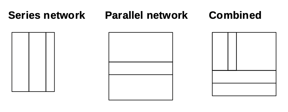
And I wrote this:

And not every resistor network can be shown as an ohmap – things outwith simple series/parallel nestings, like delta or Y networks.

It turns out I was a little hasty here. So how might ohmaps cope with more interesting networks?

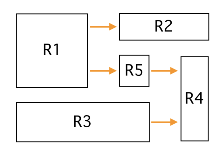
Let’s look at a simple resistor network that isn’t possible to build from just parallel and series constructions:

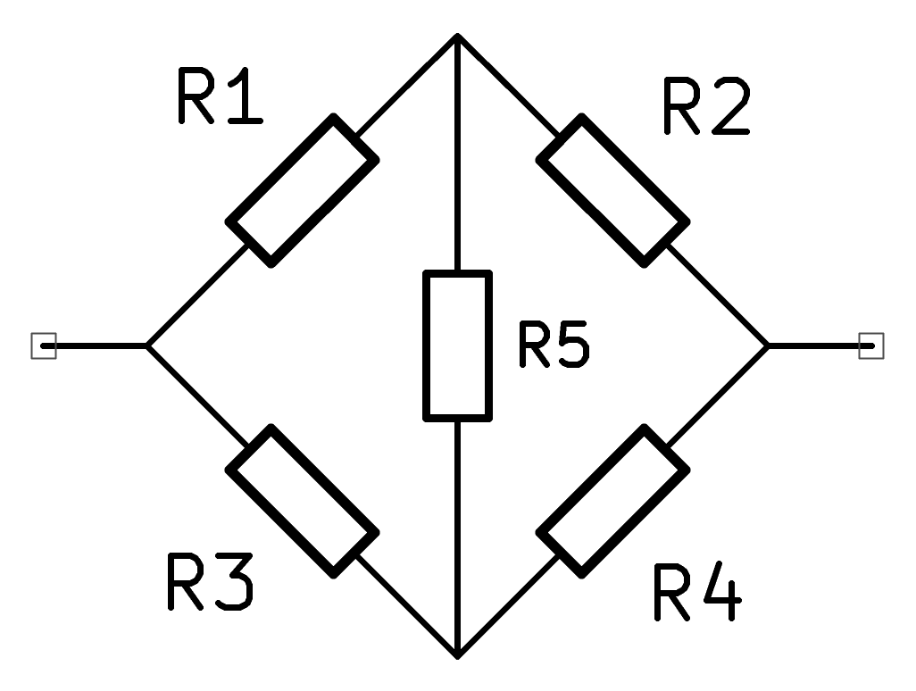
It’s very similar to a Wheatstone Bridge but with a resistor across the centre. We’ll call this network ‘W5’.

This network can’t be built from only series and parallel parts.¹

Can an ohmap represent this network?

Logically, it should be possible, because ohmaps are a way of visualising voltages and currents in a network in a way that closely ties to Kirchhoff’s V and I laws. And if you build this network and power it up, all its parts will have measurable potential differences and currents (as will the network as a whole).

Let’s make some assumptions about current: it flows left to right across the picture above, as is conventional. Then the only ambiguity is the current direction (if any) across R5. Let’s assume the resistors are chosen so that the current flows top to bottom of R5 in the diagram. Then we know the current flow in every part:

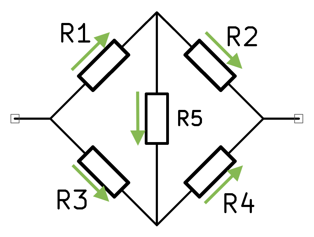
(Wheatstone bridge reminder: they work by measuring the PD² across the centre of two potential dividers. In my circuit above the current flows top-to-bottom when \(R1/R2 < R3/R4\), bottom-to-top when \(R1/R2 > R3/R4\), and no current flows when \(R1/R2 = R3/R4\) (when the bridge is balanced)).

Now we have to finagle this into an ohmap. Pen and paper seem to work best here :)

Reminders on ohmaps:

• x distances represent potential differences, with total width of diagram being the PD across the network
• y distances represent currents, with total height of diagram being the current flow into and out of the network
• current flowing from one resistor A into another B means A is directly to left of B; they overlap on the y dimension by some amount representing the current flow

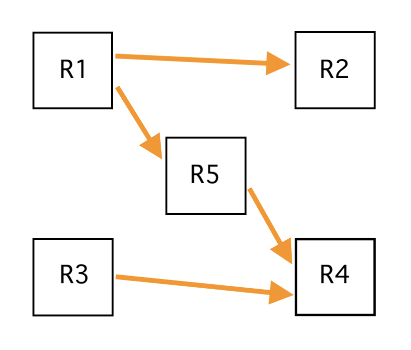
Knowing these things, we can sketch the resistors as boxes and use the arrows (showing current flow) from the earlier picture to see how the boxes need to join up in the vertical direction:

And now we move the boxes to achieve this overlap, by making the arrows all point directly to the right (and adjusting box dimensions to allow this):

Finally, removing the arrows and joining everything up, we get the general ohmap shape for our W5 circuit:

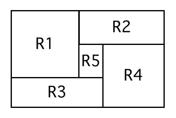
This is just a sketch and the box aspect ratios (resistances!) aren’t fine-tuned for a particular circuit.³

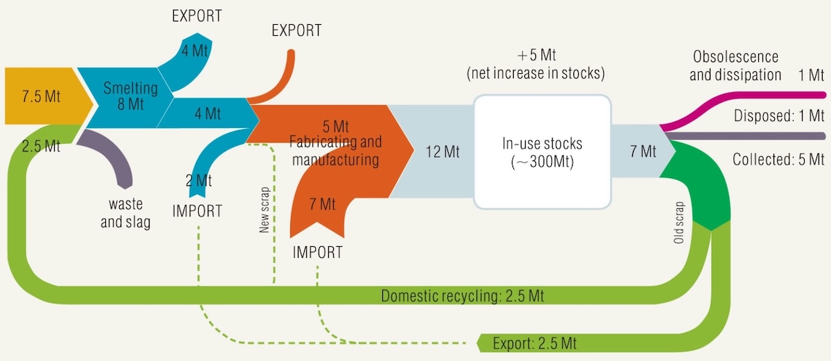
Thought: the ohmap idea isn’t that far removed from a Sankey diagram, where quantities flow from left to right, things splitting and combining:

Analysing the W5 circuit with ohmaps

How do we calculate the voltages/currents of a particular W5 circuit if we know the values of R1-R5?

The usual way to do this is to use Kirchhoff’s V and I laws: write some equations featuring voltages and currents and solve them with linear algebra.

We can do the same thing with the ohmaps by using the diagram to generate those linear equations. It’s the same trick in end, but I think it’s more intuitive to look at a picture!

So here is my version of solving W5 using an ohmap. I solve the resulting linear equation system using sympy, which I hadn’t heard much about before now; looks pretty handy to me.

But before diving into the ohmap bit, let’s remind ourselves of how solving a set linear equations works, and in particular what we need to solve a given problem. We want to know that before yanking information out of an ohmap!

Hold your nose, it’s linear algebra

There’s plenty of stuff on linear algebra out there; I’ll not repeat the basics.⁴

The interesting question here is: how many linear equations do we need so that we can solve our W5 circuit?

The circuit has five fundamental unknowns: the voltage across each resistor.

The Rouché–Capelli theorem is useful here. It tells us how many linear equations⁵ we need to solve our system: five.

So let’s find five equations. We want to find the voltages across every resistor, so we’re looking for linear equations concerning the voltages \(v_1\) to \(v_5\).

Three of the equations are quite easy to find. In ohmaps the widths of boxes correspond to voltages \(v_i\), and if we examine the ohmap picture:

we see that adding the widths of boxes 1 and 5 gives us the width of box 3:

Likewise for boxes 4, 5 and 2:

There’s another voltage sum to be had, and crucially it introduces \(v_t\) to the system, which is the total voltage across the network (ohmap picture):

This makes sense. If we want to know individual resistor voltages in this network, we need to know the total voltage across it!⁶

We still have two equations to find (to make up our five). But a) I think we’ve exhausted our options for looking at the ohmap horizontally, and b) none of the first three equations involve resistance. But the resistances have to come in somewhere!

Let’s knacker these two birds with one proverbial stone.

We can do more summing of dimensions – but vertically. The vertical dimensions in ohmaps involve current, though, not voltage.

Our linear equations are about voltages, though! What to do?

It’s \(V=IR\) to the rescue: we can restate facts about currents (I) as facts about voltages (V), because we know the resistances (R).⁷

By looking at heights of boxes we can say this about currents:

And we can rewrite these two equations using \(I = V/R\):

Ok, great, now we have five equations!

Ok, so let’s rewrite those two equations with conductance (G) instead of resistance (R), since we know that \(G = 1 / R\). Thanks, old dude in bar.

And that’s it, we now have five equations, and they all contain independent information.

Here’s our five equations all together for a selfie:

To solve this linear equation system we want to convert it into an augmented matrix, which is:

At this point you could in theory work by hand and convert the matrix to row echelon form and all that jazz.

But I’m lazy (and sensible) so I used sympy instead. Here’s the python + sympy code for solving the W5 augmented matrix given above:

from sympy import symbols, Eq, solve, factor, latex

def main():
    # resistor voltage symbols
    v1, v2, v3, v4, v5 = symbols('v1 v2 v3 v4 v5')

    # conductance symbols
    g1, g2, g3, g4, g5 = symbols('g1 g2 g3 g4 g5')

    # total voltage across network symbol
    v = symbols('v')

    # equations for solution -- we need 5 independent eqns

    eq1 = Eq(v1 - v3 + v5, 0)
    eq2 = Eq(-v2 + v4 + v5, 0)
    eq3 = Eq(v1 + v4 + v5, v)

    # two of the eqns concern current sums, rewritten as voltages (using conductance
    # instead of resistance (avoids reciprocals and hence we get simpler eqns))
    eq4 = Eq(-g1*v1 + g2*v2 + g5*v5, 0)
    eq5 = Eq(g3*v3 - g4*v4 + g5*v5, 0) # v3

    # r1, r2, r3, r4, r5 = (0.75, 3, 2, 1, 0.000000001)
    resistances = (2, 1, 5, 1.5, 0.5)
    r1, r2, r3, r4, r5 = resistances
    # substitutions. We calc conductance from resistor values
    subs = {g1: 1/r1, g2: 1/r2, g3: 1/r3, g4: 1/r4, g5: 1/r5, v: 1}

    # Solve symbolically - note we use factor() to simplify expressions
    symbolic_voltage_solutions = factor(solve([eq1, eq2, eq3, eq4, eq5], (v1, v2, v3, v4, v5), dict=True))

    # latex formatted voltage solutions
    print("$$\n\\begin{aligned}")
    for sol in symbolic_voltage_solutions:
        for var, expr in sol.items():
            equation = Eq(var, expr)
            print(f"{latex(equation)} \\\\\n\\\\")
    print("\\end{aligned}\n$$\n")

    # Evaluate each solution numerically with substituted constants

    # Verify we only have one solution as expected!
    if len(symbolic_voltage_solutions) != 1:
        print(f"Aborting, we found {len(symbolic_voltage_solutions)} solution, expected exactly one!\n")
        sys.exit(1)

    sol = symbolic_voltage_solutions[0]

    evaluated_dict_voltages = evaluate_sorted_exprs(sol, subs)
    evaluated_voltages = [value for key, value in evaluated_dict_voltages.items()]
    currents = [v / r for v, r in zip(evaluated_voltages, resistances)]

    print("\nVoltages: ", evaluated_voltages)
    print("\nCurrents: ", currents)

def sorted_values_by_key(d):
    return [value for key, value in sorted(d.items(), key=lambda item: str(item[0]))]

def evaluate_sorted_exprs(expr_dict, subs):
    sorted_items = sorted(expr_dict.items(), key=lambda item: str(item[0]))
    return {var: expr.evalf(subs=subs) for var, expr in sorted_items}

if __name__ == '__main__':
    main()

The code above

• solves the augmented matrix to give us equations for all the voltages
• outputs latex formatted equations for the solution (handy, see end of post for details)
• plugs the resistor values (and network voltage \(v_t\)) in to the derived equations to find out the voltages and currents

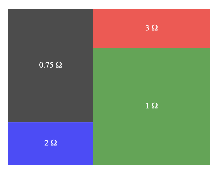
And so this code gives us the voltages and currents we need to plot an ohmap of a particular W5 circuit. Here’s an example I made using the solution from sympy:

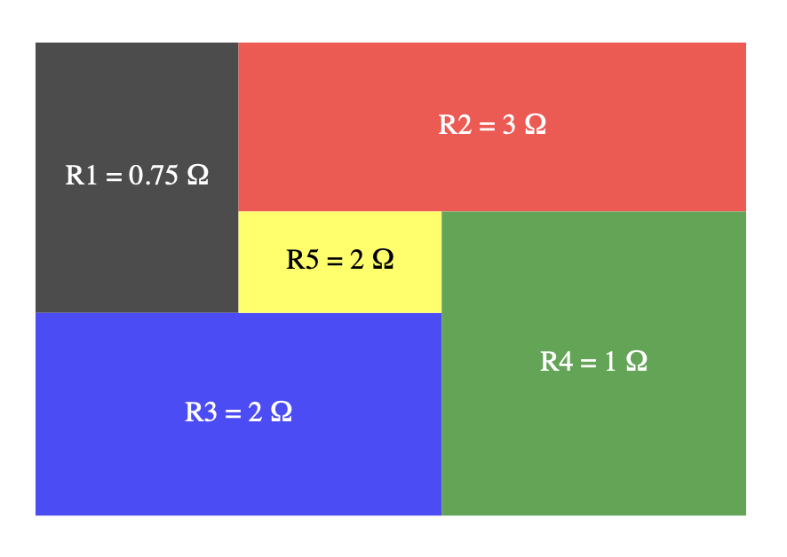
You can verify from the picture that the aspect ratios of the rectangles match the resistances. And the aspect ratio of the entire diagram, approx 1.49, is the resistance of the entire network. The width of each box represents voltage across a resistor, the height represents current flowing through a resistor.

Extreme values of \(r_5\)

There are two values for \(r_5\) that make the W5 into something familiar:

When \(r_5 = 0\), we effectively have a wire in place of \(r_5\): that’s a parallel circuit. Ohmap:

When \(r_5 = \infty\), we effectively have a open circuit (gap) in place of \(r_5\): that’s a series circuit. Ohmap:

And so, interestingly, it turns out the W5 network allows a smooth transition between series and parallel circuits (with the same four outside resistor parts), conceptually.

What does that transition actually look like in terms of the ohmap? That yellow box for \(r_5\) – how does it change between the values 0 and \(\infty\)?

We could make an animation to show this, but for now I’ve just plotted an ohmap that shows various values of \(r_5\) using outlines of boxes instead of filled colours. And we end up with this modern-art looking thing:

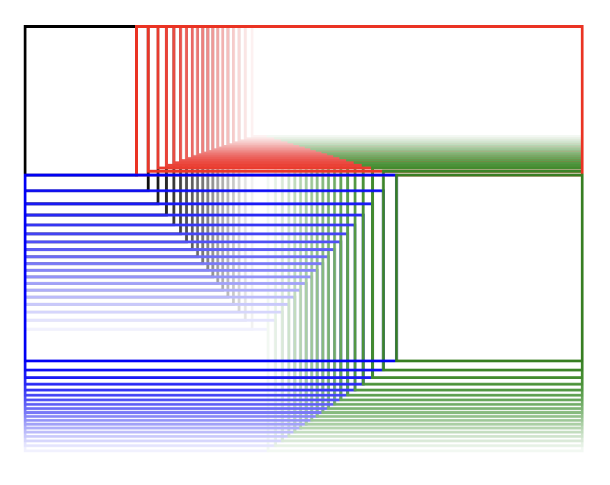
Apart from the gallery-hanging potential here, there’s some interesting to notice: the ends of lines corresponding to corners of \(r_5\) form straight paths. So this means that the corners of \(r_5\) are on a linear paths when varying only \(r_5\)).

Animation tip

To animate an ohmap with a changing a resistor value like \(r_5\), don’t just vary \(r_5\) linearly.

The most natural way is to set \(r_5 = \tan(\alpha) \) for \(0 \leq \alpha \leq 90\).

Rationale: large resistor values have to change a lot in order look much different on the ohmap.

The grim details: voltage equations

Here’s the equations for the resistor voltages as derived through sympy, using conductance instead of resistance (so \(g_i = 1 / v_i\)).

With:

we have:

A quick sanity check: \(v_5\) should be zero when \(g_1/g_3 = g_2/g_4\) as per the standard Wheatstone Bridge balance condition; and the equation for \(v_5\) is zero under that condition.   ✅

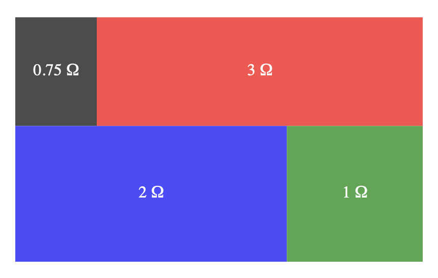
What does this all mean for photo montages?

Harking back to the original image-montage-to-resistor-network relationship:

We now know that 5 images can be arranged into a montage in the style of a W5 ohmap without squashing (aspect-changing) or cropping any of the images, allowing for an edge case: the fifth image could be close to zero-size in unlucky situations.

• Circuits
• Electronics
• Curiosities
• Ohmap